Monday, April 12, 2010
Sunday, February 14, 2010
[Activity] 8 : 3D Surface Reconstruction from Structured Light
Activity 8 : 3D Surface Reconstruction from Structured Light
In this activity, we try to reconstruct volume objects by projecting different patterns to the volume object rather than taking a stereoscopic image of the object (only 1 surface view of the object is utilizes instead of 2). This is specially useful in the field of archaeology, marine biology and other fields where non-destructive reconstruction and measuring techniques for artifacts are needed.
The following image shows the setup for this technique.

Setup: (a) projector, (b) camera [1]
Here, instead of two cameras, the method utilizes a camera and a projector. The distance between the camera and the projector is known, as well as the distance between the camera and the object being measure. In addition, the focal points of the camera has already been pre-measured.
The patterns to be projected to a volume object is a set binary gray code images. The images projected to the object volume is shown below.

Binary images projected to the volume object
These binary code images, which can also be treated as logical matrices, will then be multiplied with increasing powers of two. After each pattern is multiplied by a power of two, the resulting matrix will be added to other resulting matrices to come up with a matrices with its column values unique. This process is illustrated below.

Binary images to graycode matrix [1]
For this activity, the volume object used is a rectangular pyramid. The resulting images are shown below.

Patterns projected to the volume image
The resulting binary code images, for both reference plane and object planes, are shown below.
For the reference plane, noise and inaccuracies in the grayscale to BW conversion resulted to noisy (or warping) columns. To fix this, the first row was assumed to be accurate and used as a base for other rows. The result was a matrix with more distinct columns.
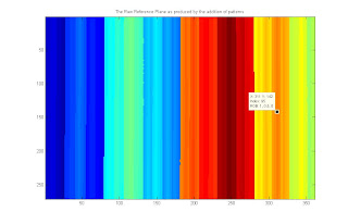
Reference plane as produced by adding the gray coded binary images
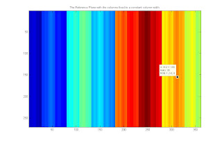
The reference plane fixed by setting all the rows equal to the first row
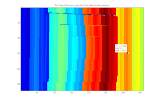
The object plane produces by adding the gray coded binary images
projected to the volume object
The reconstruction of the volume object roots from the fact that when a volume object was projected with the binary patterns, the patterns will be distorted proportional to the contours and height of the object. It can be verified by looking into the object plane image above and comparing it to the reference plane. The shape of the object volume can be visually reconstructed based from the distortions of the different columns. This is the theory behind 3d reconstruction from binary images.
Shown below is the illustration on how the algorithm derives the height of an object based upon the distortion of a column.

Height derivation from column distortion [1]
Using the concept of similar triangles and the focal length which is unique for the camera used, the following equations show how to get the height.

Equations to solve for height 'z'
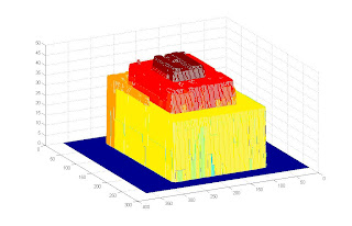
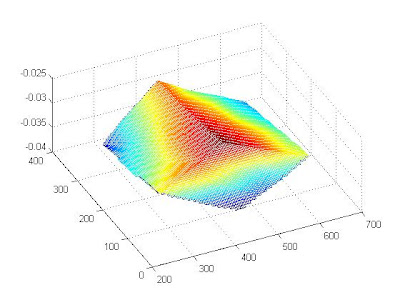
The images below show the resulting reconstruction. The first image is the raw reconstruction. Since the input images aren't perfect (note the shadows in the top portion of the pyramid), extreme values can be obtained resulting to erroneous height calculations. This was corrected by utilizing prior knowledge about the volume. Since we know that the middle part is the highest portion, we remove all heights that are higher than the middle portion of the pyramid. A 2-dimensional median filter is then utilized to even out the heights.
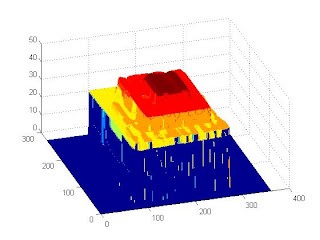
Raw object volume reconstruction
Reconstructed object volume further processed
We can see that the final reconstructions still has variation in height, especially in the first level. This can be traced due to the variation in the lighting present in the images where the patterns were projected to the volume. Below is one of the images.

Green box area: Area where light seem to flash out the black stripes
We can see that the portion highlighted by the box shows some of the black columns are not as black or emphasized as those in the upper portion of the volume. This would have an effect when the image is converted into a logical image as the columns of zeros and ones would not be as distinct. This is similar to the raw reference plane that we have seen above. Since the columnsa aren't as solid as planned, distortions would appear.
Still, the reconstructed volume is very similar to the object volume and we could conclude that the method works.
Code Listing:
function cropall
%
gthresh = 0.6;
width = 360;
height = 270;
refplaneraw = zeros(height+1, width+1);
objectplane = refplaneraw;
% rect = [470 310 width height];
levels = 7;
for i=1:1:levels
reffile = strcat('newrefimage_', num2str(i), '.jpg');
objfile = strcat('newimage_', num2str(i), '.jpg');
refimage = imread(reffile);
objimage = imread(objfile);
% newimage = imcrop(temp, rect);
gthreshobj = graythresh(objimage);
gthreshref = graythresh(refimage);
BWrefimage = im2bw(refimage, gthreshref);
BWobjimage = im2bw(objimage, gthreshobj);
objectplane = objectplane + double(BWobjimage*(2^(levels-i)));
refplaneraw = refplaneraw + double(BWrefimage*(2^(levels-i)));
end
refline = refplaneraw(1,:);
refplanefixed = refplaneraw;
for i=1:1:size(refplanefixed ,1)
refplanefixed (i,:) = refline;
end
close all
figure, imagesc(refplaneraw);
title('The Raw Reference Plane as produced by the addition of patterns');
figure, imagesc(refplanefixed);
title('The Reference Plane with the columns fixed to a constant column width');
figure, imagesc(objectplane);
title('The Object Plane as produced by the addition of the patterns');
save patterns.mat refplaneraw refplanefixed objectplane
%% %
load patterns.mat
close all
Ck = 3.2; % focal length
L = 67; % camera to reference plane distance
B = 16; % camera to projector distance
refplanefixed = refplaneraw;
columnlabels = unique(refplanefixed(1,:));
newobjectplane = zeros(size(objectplane, 1), size(objectplane, 2));
for i=1:1:length(columnlabels)
[y, xobj] = find(objectplane == columnlabels(i));
[ytemp, xref] = find(refplanefixed == columnlabels(i)); % OK
rowlabels = unique(y);
for j=1:1:length(rowlabels)
% find the x-coordinates given y-coordinate
x_obj = xobj(find(y == rowlabels(j))); % xcords in the object plane
x_ref = xref(find(ytemp == rowlabels(j))); % xcords in the reference plane
if max(x_obj) > max(x_ref)
UV = (min(x_obj) - min(x_ref)) .* Ck;
newval = (L * UV)./ (B + UV);
for k=1:1:length(x_obj)
newobjectplane(rowlabels(j), x_obj(k)) = newval;
end
end
end
end
newobjectplane = newobjectplane .* (newobjectplane > 0);
newobjectplane1 = newobjectplane;
newobjectplane1(find(newobjectplane > 47.3)) = 0;
newobjectplane2 = medfilt2(newobjectplane1, [10 10]);
figure,mesh(newobjectplane)
figure,mesh(newobjectplane1)
figure,mesh(newobjectplane2)
I give myself a grade of 9.5 for this activity for completing the objectives but not coming up with a perfect reconstruction though by "cleaning" the first reconstruction, a better image was achieved.
References:
[1] "Volume Estimation from Partial View through Graycode Illumination", K. Vergel and M. Soriano, SPP (Samahang Pisika ng Pilipinas) Slide Show Presentation, National Institute of Physics, University of the Philippines - Diliman
[2] Activity 8 - 3D Surface Reconstruction from Structured Light, M. Soriano, Physics 305 Activity Sheet
[Activity] 7 : Stereometry
Activity 7 : Stereometry
For this activity, we would construct a 3-d image of a volume object given some of its 2D images/views. The image/views should have little differences in the position of the pixels. These small differences would be used to calculate depth information, information that will add an additional dimension to the 2D image.
We start with the following 2 input images of the same object. It is assumed that the vertical position of the pixels remain the same and the change only comes from the horizontal position pof the pixels.

Input images
The following illustration shows how the depth can be computed from the difference of the location of a certain pixel. Here, we know the difference in the distance (b), the focal length of the camera that we used (f) and the pixel locations of a point in the image (x1, x2)

The following equation show how, from the difference in coordinate values of the pixel, we could compute the depth 'z'. We use here the theory behind similar triangles.

Equations to calculate for depth
After doing the calculations, the computed 3D image for the 2 input images above are shown below. It seems that the corners has been properly reconstructed though the sides of the cube aren't as planar as hoped. This can be accounted to less than perfect matching of the pixels in the first and second image.
Final 3D reconstruction image
Code Listing
function stiryo
load calibdata;
b = 2.54; % the length between two points, 1 inch
Aparams = reshape(A, 3, 4);
Amat = Aparams(1:3,1:3);
Aparams = rq(Amat);
K = Aparams ./ Aparams(3,3);
focal = K(2,2) / K(1,1);
bf = b * focal;
image1 = imread('im1.jpg');
image2 = imread('im2.jpg');
newimage = zeros(size(image1));
% for i=1:1:37
imshow(image1);
[x1, y1] = ginput
close all
imshow(image2);
[x2, y2] = ginput
close all
% end
save
load cubecoords.mat
x1 = round(x1);
x2 = round(x2);
y1 = round(y1);
x = linspace(min(x1), max(x1), 100);
y = linspace(min(y1), max(y1), 100);
[X, Y] = meshgrid(x,y);
z = bf ./ (x2 - x1);
Z = griddata(x1,y1,z,X,Y,'linear');
size(X)
size(Y)
size(Z)
mesh(X,Y,Z)
end
I give myself a grade of 9.5 for this activity for achieving the objectives but wasn't able to get perfect results. The sides are not as perfectly flat as desired.
References
[1] Activity 7: Stereometry Activity Sheet, M. Soriano, Physics 305
[Activity] 6 : Camera Calibration
Activity 6 : Camera Calibration
For this activity, we try to extract the intrinsic and extrinsic characteristics of a camera. Even if two cameras are of the same brand and model, their characteristics still differ minutely. We extract these characteristics by utilizing two boards with a pattern similar to chess board, the first being a single plane board and the second having a 90-degree angle in the middle of the board. The latter board is called the Tsai board, named from Roger Tsai. These two boards are shown below.

Boards used to calibrate the camera, (left) planar and (right) Tsai
I. Using a folded checkboard (Tsai Board)
Using the Tsai board and a predefined axis, we sample pixels in the Tsai board image that corresponds to the square corners. The result will be a matching between the coordinates of the corner pixels and the coordinates of the defined axis. The values will then be used in the following equation:

Equation relating the image pixel coordinates to the
defined (x,y,z) coordinates
The vector of a's can be computed by using the following equation.

Equation to solve for vector 'a'
The vector a represents the intrinsic and extrinsic characteristics of the camera. Using these values, we could predict any other point in the image by using the following formula:
 Equations to predict other image coordinates xi's and yi's
The following shows the input and output of this part of the activity. In the left image, the green crosshairs shows the corners that have been selected to compute for the intrinsic/extrinsic characteristics of the camera. The image on the right shows that the other corners have been properly predicted.

(Left) Selected points and (Right) Rest of the points properly predicted.
II. Using a camera calibration toolbox
Using the camera calibration toolbox, instead of specifying many square corners, we only need to specify the four cornermost points in the planar board and let the program detect the lines and corners of the image. Aside from the corners, the program also detects if warping is present.
The following images show the board with the corners detected.


And most importantly, the program computed the intrinsic and extrinsic characteristics as shown below.

Calibration values as computed by the Calibration Toolbox
Code Listing
function tsaiboard
board = imread('tsai.jpg');
figure,imshow(board);
xi = [];
yi = [];
xyz = [];
for ytemp=0:2:10
xyz = [xyz ; [0 ytemp 0]];
disp([0 ytemp 0]);
[x, y] = ginput;
xi = [xi x(end)];
yi = [yi y(end)];
end
for ytemp=0:2:10
for xz=1:2:7
xyz = [xyz ; [xz ytemp 0]];
disp([xz ytemp 0]);
[x, y] = ginput;
xi = [xi x(end)];
yi = [yi y(end)];
end
for xz=1:2:7
xyz = [xyz ; [0 ytemp xz]];
disp([0 ytemp xz]);
[x, y] = ginput;
xi = [xi x(end)];
yi = [yi y(end)];
end
end
save 'coords.mat';
load coords.mat;
Q = [];
p = [];
for i=1:1:size(xyz, 1)
currentxyz = xyz(i,:);
currentQ = [currentxyz 1 0 0 0 0 -(xi(i)*currentxyz(1)) -(xi(i)*currentxyz(2)) -(xi(i)*currentxyz(3)); 0 0 0 0 currentxyz 1 -(yi(i)*currentxyz(1)) -(yi(i)*currentxyz(2)) -(yi(i)*currentxyz(3))];
% pause
Q = [Q; currentQ];
p = [p; xi(i); yi(i)];
end
A = inv(Q'*Q)*Q'*p
save coords.mat;
figure, imshow(imread('tsai.jpg'));
hold
for ytemp=0:1:10
for xz=1:1:7
xi = round((A(1)*xz + A(2)*ytemp + A(3)*0 + A(4))/(A(9)*xz + A(10)*ytemp + A(11)*0 + 1));
yi = round((A(5)*xz + A(6)*ytemp + A(7)*0 + A(8))/(A(9)*xz + A(10)*ytemp + A(11)*0 + 1));
disp([xi yi]);
plot(xi, yi, '+', 'color', 'green');
end
for xz=1:1:7
xi = round((A(1)*0 + A(2)*ytemp + A(3)*xz + A(4))/(A(9)*0 + A(10)*ytemp + A(11)*xz + 1));
yi = round((A(5)*0 + A(6)*ytemp + A(7)*xz + A(8))/(A(9)*0 + A(10)*ytemp + A(11)*xz + 1));
disp([xi yi]);
plot(xi, yi, '+', 'color', 'green');
end
end
I give myself a grade of 8.5 for this activity for successfully accomplishing the objectives. However, I could not compare the extrinsic/intrinsic values of the camera for both methods. I don't know which variables to compare.
References:
[1] Activity 6: Camera Calibration Activity Sheet, Maricor Soriano
[2] Camera Calibration Toolbox, Available: http://www.vision.caltech.edu/bouguetj/calib_doc/
[Activity] 5 : Shape from Texture
Activity 5 : Shape from Texture
In this activity, we try to reconstruct 3-dimensional surfaces based on their texture. Textures in objects can be constant or have a repeating pattern. These can be utilized to reconstruct the surface without the need for other information.
For example, for the the image below:

Sample object with periodic texture pattern [1]
We could easily reconstruct the contour of the image as round (most likely it is a pipe). We could say this as we reconstruct the contour based on what we see, pattern that become distorted on the sides. We could do this even though what we have is only a 2-dimensional, BW image.
For us to implement this on a computer, we utilize a set of functions called the Gabor Filters. Gabor Filters are Gaussian kernel functions modulated by a complex sinusoid. [2] For this activity, a bank of Gabor Filters with specific angles and frequencies are used. These functions will be convolved with the original image to extract the orientations information based on the patterns/texture that can be seen in the object. The frequencies and angles that were used in the Gabor Filter bank are shown below.

Angles and Frequencies used in the Gabor Filter Bank [1]
The rest of the steps are shown in the image below.

Steps in reconstructing 3D contours based texture [1]
An example input image is shown below. It is a ball covered with white polka dots on a black background. We would try to reconstruct the contour based on its texture. The image was already converted into grayscale.
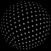
Ball with white spots as texture
Based on the steps above, the reconstructed image and its needle plot is shown below.

The reconstructed surface of the ball and its needle plot
Some more examples.


Code Listing:
function texture3d
texture = imread('coral1.jpg');
[m n] = size(size(texture));
if n == 3
texture = rgb2gray(texture);
end
min_dimension = min(size(texture));
resize_factor = min_dimension/150;
im = imresize(texture, 1/resize_factor);
% im = texture;
% flags/values
A = zeros(size(im));
B = zeros(size(im));
C = zeros(size(im));
totalA = zeros(size(im));
values = [12 16.97 24 33.94 48 67.882 96];
for angle=-70:20:90
for k = 1:1:7
[angle values(k)]
wavelength = values(k);
spatialgabor2(im, wavelength, deg2rad(angle));
[Aim, Bim, Cim] = spatialgabor2(im, wavelength, deg2rad(angle));
totalA = totalA + (Aim.^2);
A = A + ((Bim.^2)./(4*pi^2));
B = B + 2.*((Bim.*Cim)./(4*pi^2));
C = C + ((Cim.^2)./(4*pi^2));
end
end
A = A ./ totalA;
B = B ./ totalA;
C = C ./ totalA;
firstterm = A + C;
secondterm = sqrt(B.^2 + (A - C).^2);
M = 0.5 .* (firstterm + secondterm);
m = 0.5 .* (firstterm - secondterm);
theta = 0.5 .* (atan(B ./ (A - C)));
save data
Mm = sqrt(M .* m);
[x, y] = find(Mm == min(Mm(:)));
x0 = x(1);
y0 = y(1);
Ms = M(x0, y0);
ms = m(x0, y0);
slant = acos(sqrt((Ms*ms)./(M.*m)));
tilt = theta - (0.5 .* (acos((((((cos(slant)).^2) + 1) .* (M + m)) - (2*(Ms + ms)))...
./((sin(slant .* (M - m))).^2))));
% tilt = (((((cos(slant)).^2) + 1) .* (M + m)) - (2*(Ms + ms)))...
% ./((sin(slant .* (M - m))).^2);
tilt(isnan(tilt)) = 0;
save data
load data;
figure, needleplotst(abs(slant), abs(tilt), 20, 4); title('needle plot');
recsurf = shapeletsurf(abs(slant), abs(tilt), 6, 1, 2, 'tiltamb');
figure, mesh(-recsurf(1:130,:)); title('integrated surface');
% save data
function [A, B, C] = spatialgabor2(im, wavelength, angle)
% function spatialgabor2(im, wavelength, angle)
im = double(im);
% % Construct Gabor filters
b = 1; % bandwidth in one-octave
sigma = ((1/pi)*(sqrt(log(2)/2))*(2^b + 1)/(2^b - 1))*wavelength; % space constant
[x,y] = meshgrid(-sigma+1:sigma); % size of the Gabor filter
gaborFilter = (1/(2*pi*(sigma.^2))).* (exp(-((x.*cos(angle) + y.*sin(angle)).^2 ...
+ (-x.*sin(angle) + y.*cos(angle)).^2)/(2.*sigma^2)))...
.* (cos((2*pi*(1/wavelength)).*(x*cos(angle) + y*sin(angle))));
gaborpartialx = (exp(((x.*cos(angle) + y.*sin(angle))^2./2 + (y.*cos(angle) - x.*sin(angle))^2./2)./(2.*sigma^2)).*cos((2.*pi.*(x.*cos(angle) + y.*sin(angle)))./wavelength).*(cos(angle).*(x.*cos(angle) + y.*sin(angle)) - sin(angle).*(y.*cos(angle) - x.*sin(angle))))./(4.*pi.*sigma^4) - (exp(((x.*cos(angle) + y.*sin(angle))^2./2 + (y.*cos(angle) - x.*sin(angle))^2./2)./(2.*sigma^2)).*sin((2.*pi.*(x.*cos(angle) + y.*sin(angle)))./wavelength).*cos(angle))./(sigma^2.*wavelength);
gaborpartialy = (exp(((x.*cos(angle) + y.*sin(angle))^2./2 + (y.*cos(angle) - x.*sin(angle))^2./2)./(2.*sigma^2)).*cos((2.*pi.*(x.*cos(angle) + y.*sin(angle)))./wavelength).*(cos(angle).*(y.*cos(angle) - x.*sin(angle)) + sin(angle).*(x.*cos(angle) + y.*sin(angle))))./(4.*pi.*sigma^4) - (exp(((x.*cos(angle) + y.*sin(angle))^2./2 + (y.*cos(angle) - x.*sin(angle))^2./2)./(2.*sigma^2)).*sin((2.*pi.*(x.*cos(angle) + y.*sin(angle)))./wavelength).*sin(angle))./(sigma^2.*wavelength);
% % construct gaussian filter
[rowsize colsize] = size(im);
filt_size = fix((min(rowsize, colsize)) * 0.15);
f_gauss = fspecial('gaussian', [filt_size filt_size], filt_size-10);
A = abs(conv2(im, gaborFilter, 'same'));
B = imfilter(abs(conv2(im, gaborpartialx, 'same')), f_gauss, 'same');
C = imfilter(abs(conv2(im, gaborpartialy, 'same')), f_gauss, 'same');
% figure,imagesc(gaborFilter);
end
I give myself a grade of 10 for this activity for successfully implementing the steps and implementing it correctly to a number of textures.
References:
[1] "Shape from Texture from Local Spectral Moments," B.J. Super, A.C. Bovik, IEEE Transactions on Pattern Recognition and Machine Intelligence, Vol. 17. No. 14, 1995
[2] "Tutorial on Gabor Filters," Available: http://mplab.ucsd.edu/tutorials/gabor.pdf
[3] "Matlab and Octave Functions for Computer Vision and Image Processing," Peter Kovesi, Available:http://www.csse.uwa.edu.au/~pk/Research/MatlabFns/
[Activity] 4 : High Dynamic Range Imaging
Activity 4 : High Dynamic Range Imaging
In this activity, we took pictures of a high-intensity scene or object, plasma sheets to be specific. Each picture (assuming that the image has constant brightness throughout the data gathering) was taken with different exposure time. The objective for this activity is to utilize all the pictures, having different exposure times, and come up with a new image that will provide more detail as compared to the detail available to each individual image.
The following are the input images (plasma sheets) used in this activity with their corresponding exposure time (in seconds).

Input Images: Top row: (a) 1/125, (b) 1/200, (c) 1/320, (d) 1/500
Bottom row: (e) 1/640 , (f) 1/800 , (g) 1/1000
From the input images, several points were chosen and their values was plotted against the changing exposure time. We could see from the graph below the relationship between the recorded intensity of the plasma sheet and the log of the length of the exposure time for that certain image.
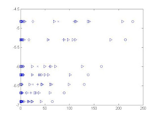
Intensity value vs. Log exposure plot
The program was coded to randomly pick 1000 points (arbitrary number) and record the intensity values. This was then fed to the code given by Debevec and Malik [1] in order to solve for log exposure (g) and the log film irradiance (lE).
The plot of g is shown below.
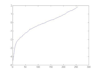
Log exposure plot
After the function (g) was obtained, we pick any of the input images and replace the intensity values in the image with new values depending on the function (g) and the image's exposure time. The output of the program, in grayscale, is shown below, beside it is the brightest of all the input images.

Left: High Dynamic Range Image, Right: Brightest input image
We could see here that the high dynamic range image offers more details compared to the brightest image. Focus on the details in the rim and we could see that the screws are more highlighted. To see more details of the plasma sheet (as we could see nothing much about the plasma sheet here), the image was re-rendered using imagesc. The resulting image is shown below.
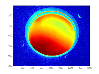
High dynamic range image using imagesc
Code Listing:
function hdr
% data
deltaT = 1./ [125 200 400 500 640 800 1000];
numpoints = 1000;
numrows = fix(rand(numpoints,1)*(1200-1))+1;
numcols = fix(rand(numpoints,1)*(1600-1))+1;
image_points = [numrows numcols];
% image_points = [510 875; %ok
% 606, 318;
% 540, 630;
% 942, 642;
% 790, 600; %ok
% 690 800]; %ok
% B(j) is the log delta t, or log shutter speed, for image j
Bj = log(deltaT);
% Z(i,j) is the pixel values of pixel location number i in image j
num_exposures = 7;
num_points = size(image_points, 1);
Zij = ones(num_points, num_exposures);
for i=1:1:num_exposures
filename = strcat(num2str(i), '.jpg');
current_image = rgb2gray(imread(filename));
for j=1:1:num_points
Zij(j,i) = current_image(image_points(j,1), image_points(j,2));
end
end
close all
for i=1:1:num_points
switch i
case 1
pattern = '+';
case 2
pattern = 'x';
case 3
pattern = 'o';
case 4
pattern = 's';
case 5
pattern = 'd';
case 6
pattern = '<';
case 7
pattern = '>';
end
plot(Zij(i,:)',Bj, pattern);
hold on
end
%
save data2.mat Zij Bj
load data2.mat
l = 10;
close all
[g,lE]=gsolve(Zij,Bj,l,@w);
image1 = rgb2gray(imread('1.jpg'));
new_hdr = uint8(zeros(size(image1)));
for i=1:1:7
current_file = rgb2gray(imread(strcat(num2str(i), '.jpg')));
new_hdr = new_hdr + current_file;
end
new_hdr = new_hdr ./ i;
% figure, imshow(new_hdr);
lnEi_temp = g(image1(:)+1) + Bj(1);
lnEi = reshape(lnEi_temp, size(image1,1), size(image1,2));
imwrite(uint8(lnEi), 'output.jpg');
figure,imshow(lnEi, []);
colormap(gray);
figure, imagesc(lnEi);
figure, plot(g);
end
% gsolve.m ? Solve for imaging system response function
%
% Given a set of pixel values observed for several pixels in several
% images with different exposure times, this function returns the
% imaging system’s response function g as well as the log film irradiance
% values for the observed pixels.
%
% Assumes:
%
% Zmin = 0
% Zmax = 255
%
% Arguments:
%
% Z(i,j) is the pixel values of pixel location number i in image j
% B(j) is the log delta t, or log shutter speed, for image j
% l is lamdba, the constant that determines the amount of smoothness
% w(z) is the weighting function value for pixel value z
%
% Returns:
%
% g(z) is the log exposure corresponding to pixel value z
% lE(i) is the log film irradiance at pixel location i
%
function [g,lE]=gsolve(Z,B,l,w)
n = 256;
A = zeros(size(Z,1)*size(Z,2)+n+1,n+size(Z,1));
b = zeros(size(A,1),1);
%% Include the data?fitting equations
k = 1;
for i=1:size(Z,1)
for j=1:size(Z,2)
wij = w(Z(i,j)+1);
A(k,Z(i,j)+1) = wij; A(k,n+i) = -wij; b(k,1) = wij * B(j);
k=k+1;
end
end
%% Fix the curve by setting its middle value to 0
A(k,129) = 1;
k=k+1;
%% Include the smoothness equations
for i=1:n-2
A(k,i)=l*w(i+1); A(k,i+1)=-2*l*w(i+1); A(k,i+2)=l*w(i+1);
k=k+1;
end
%% Solve the system using SVD
x = A\b;
g = x(1:n);
lE = x(n+1:size(x,1));
function d = w(Zint)
Zmin = 1;
Zmax = 255;
Zmid = (Zmin + Zmax)/2.0;
if Zint <= Zmid
d = (Zint - Zmin);
else
d = (Zmax - Zint);
end
return;
I give myself a grade of 10 for accomplishing the objectives and learning how to pass functions in Matlab. (yey! =)
References:
[1] "Recovering High Dynamic Range Radiance Maps from Photographs," P.E. Debevec, J. Malik, University of California, Berkeley
[2] High Dynamic Range Activity Sheet, Dr. Maricor Soriano
Subscribe to:
Posts (Atom)