[Activity] 5 : Shape from Texture

Activity 5 : Shape from Texture

In this activity, we try to reconstruct 3-dimensional surfaces based on their texture. Textures in objects can be constant or have a repeating pattern. These can be utilized to reconstruct the surface without the need for other information.

For example, for the the image below:

Sample object with periodic texture pattern [1]

We could easily reconstruct the contour of the image as round (most likely it is a pipe). We could say this as we reconstruct the contour based on what we see, pattern that become distorted on the sides. We could do this even though what we have is only a 2-dimensional, BW image.

For us to implement this on a computer, we utilize a set of functions called the Gabor Filters. Gabor Filters are Gaussian kernel functions modulated by a complex sinusoid. [2] For this activity, a bank of Gabor Filters with specific angles and frequencies are used. These functions will be convolved with the original image to extract the orientations information based on the patterns/texture that can be seen in the object. The frequencies and angles that were used in the Gabor Filter bank are shown below.

Angles and Frequencies used in the Gabor Filter Bank [1]

The rest of the steps are shown in the image below.

Steps in reconstructing 3D contours based texture [1]

An example input image is shown below. It is a ball covered with white polka dots on a black background. We would try to reconstruct the contour based on its texture. The image was already converted into grayscale.

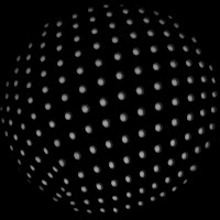
Ball with white spots as texture

Based on the steps above, the reconstructed image and its needle plot is shown below.

The reconstructed surface of the ball and its needle plot

Some more examples.

Code Listing:

function texture3d

texture = imread('coral1.jpg');

[m n] = size(size(texture));

if n == 3

texture = rgb2gray(texture);

end

min_dimension = min(size(texture));

resize_factor = min_dimension/150;

im = imresize(texture, 1/resize_factor);

% im = texture;

% flags/values

A = zeros(size(im));

B = zeros(size(im));

C = zeros(size(im));

totalA = zeros(size(im));

values = [12 16.97 24 33.94 48 67.882 96];

for angle=-70:20:90

for k = 1:1:7

[angle values(k)]

wavelength = values(k);

spatialgabor2(im, wavelength, deg2rad(angle));

[Aim, Bim, Cim] = spatialgabor2(im, wavelength, deg2rad(angle));

totalA = totalA + (Aim.^2);

A = A + ((Bim.^2)./(4*pi^2));

B = B + 2.*((Bim.*Cim)./(4*pi^2));

C = C + ((Cim.^2)./(4*pi^2));

end

end

A = A ./ totalA;

B = B ./ totalA;

C = C ./ totalA;

firstterm = A + C;

secondterm = sqrt(B.^2 + (A - C).^2);

M = 0.5 .* (firstterm + secondterm);

m = 0.5 .* (firstterm - secondterm);

theta = 0.5 .* (atan(B ./ (A - C)));

save data

Mm = sqrt(M .* m);

[x, y] = find(Mm == min(Mm(:)));

x0 = x(1);

y0 = y(1);

Ms = M(x0, y0);

ms = m(x0, y0);

slant = acos(sqrt((Ms*ms)./(M.*m)));

tilt = theta - (0.5 .* (acos((((((cos(slant)).^2) + 1) .* (M + m)) - (2*(Ms + ms)))...

./((sin(slant .* (M - m))).^2))));

% tilt = (((((cos(slant)).^2) + 1) .* (M + m)) - (2*(Ms + ms)))...

% ./((sin(slant .* (M - m))).^2);

tilt(isnan(tilt)) = 0;

save data

load data;

figure, needleplotst(abs(slant), abs(tilt), 20, 4); title('needle plot');

recsurf = shapeletsurf(abs(slant), abs(tilt), 6, 1, 2, 'tiltamb');

figure, mesh(-recsurf(1:130,:)); title('integrated surface');

% save data

function [A, B, C] = spatialgabor2(im, wavelength, angle)

% function spatialgabor2(im, wavelength, angle)

im = double(im);

% % Construct Gabor filters

b = 1; % bandwidth in one-octave

sigma = ((1/pi)*(sqrt(log(2)/2))*(2^b + 1)/(2^b - 1))*wavelength; % space constant

[x,y] = meshgrid(-sigma+1:sigma); % size of the Gabor filter

gaborFilter = (1/(2*pi*(sigma.^2))).* (exp(-((x.*cos(angle) + y.*sin(angle)).^2 ...

+ (-x.*sin(angle) + y.*cos(angle)).^2)/(2.*sigma^2)))...

.* (cos((2*pi*(1/wavelength)).*(x*cos(angle) + y*sin(angle))));

gaborpartialx = (exp(((x.*cos(angle) + y.*sin(angle))^2./2 + (y.*cos(angle) - x.*sin(angle))^2./2)./(2.*sigma^2)).*cos((2.*pi.*(x.*cos(angle) + y.*sin(angle)))./wavelength).*(cos(angle).*(x.*cos(angle) + y.*sin(angle)) - sin(angle).*(y.*cos(angle) - x.*sin(angle))))./(4.*pi.*sigma^4) - (exp(((x.*cos(angle) + y.*sin(angle))^2./2 + (y.*cos(angle) - x.*sin(angle))^2./2)./(2.*sigma^2)).*sin((2.*pi.*(x.*cos(angle) + y.*sin(angle)))./wavelength).*cos(angle))./(sigma^2.*wavelength);

gaborpartialy = (exp(((x.*cos(angle) + y.*sin(angle))^2./2 + (y.*cos(angle) - x.*sin(angle))^2./2)./(2.*sigma^2)).*cos((2.*pi.*(x.*cos(angle) + y.*sin(angle)))./wavelength).*(cos(angle).*(y.*cos(angle) - x.*sin(angle)) + sin(angle).*(x.*cos(angle) + y.*sin(angle))))./(4.*pi.*sigma^4) - (exp(((x.*cos(angle) + y.*sin(angle))^2./2 + (y.*cos(angle) - x.*sin(angle))^2./2)./(2.*sigma^2)).*sin((2.*pi.*(x.*cos(angle) + y.*sin(angle)))./wavelength).*sin(angle))./(sigma^2.*wavelength);

% % construct gaussian filter

[rowsize colsize] = size(im);

filt_size = fix((min(rowsize, colsize)) * 0.15);

f_gauss = fspecial('gaussian', [filt_size filt_size], filt_size-10);

A = abs(conv2(im, gaborFilter, 'same'));

B = imfilter(abs(conv2(im, gaborpartialx, 'same')), f_gauss, 'same');

C = imfilter(abs(conv2(im, gaborpartialy, 'same')), f_gauss, 'same');

% figure,imagesc(gaborFilter);

end

I give myself a grade of 10 for this activity for successfully implementing the steps and implementing it correctly to a number of textures.

References:

[1] "Shape from Texture from Local Spectral Moments," B.J. Super, A.C. Bovik, IEEE Transactions on Pattern Recognition and Machine Intelligence, Vol. 17. No. 14, 1995

[2] "Tutorial on Gabor Filters," Available: http://mplab.ucsd.edu/tutorials/gabor.pdf

[3] "Matlab and Octave Functions for Computer Vision and Image Processing," Peter Kovesi, Available:http://www.csse.uwa.edu.au/~pk/Research/MatlabFns/