[Activity] 4 : High Dynamic Range Imaging

Activity 4 : High Dynamic Range Imaging

In this activity, we took pictures of a high-intensity scene or object, plasma sheets to be specific. Each picture (assuming that the image has constant brightness throughout the data gathering) was taken with different exposure time. The objective for this activity is to utilize all the pictures, having different exposure times, and come up with a new image that will provide more detail as compared to the detail available to each individual image.

The following are the input images (plasma sheets) used in this activity with their corresponding exposure time (in seconds).

Input Images: Top row: (a) 1/125, (b) 1/200, (c) 1/320, (d) 1/500

Bottom row: (e) 1/640 , (f) 1/800 , (g) 1/1000

From the input images, several points were chosen and their values was plotted against the changing exposure time. We could see from the graph below the relationship between the recorded intensity of the plasma sheet and the log of the length of the exposure time for that certain image.

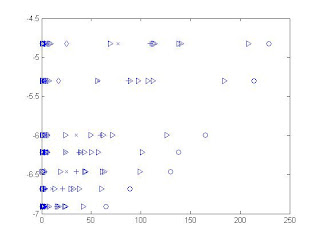
Intensity value vs. Log exposure plot

The program was coded to randomly pick 1000 points (arbitrary number) and record the intensity values. This was then fed to the code given by Debevec and Malik [1] in order to solve for log exposure (g) and the log film irradiance (lE).

The plot of g is shown below.

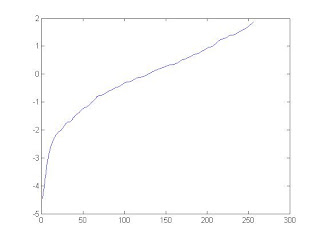
Log exposure plot

After the function (g) was obtained, we pick any of the input images and replace the intensity values in the image with new values depending on the function (g) and the image's exposure time. The output of the program, in grayscale, is shown below, beside it is the brightest of all the input images.

Left: High Dynamic Range Image, Right: Brightest input image

We could see here that the high dynamic range image offers more details compared to the brightest image. Focus on the details in the rim and we could see that the screws are more highlighted. To see more details of the plasma sheet (as we could see nothing much about the plasma sheet here), the image was re-rendered using imagesc. The resulting image is shown below.

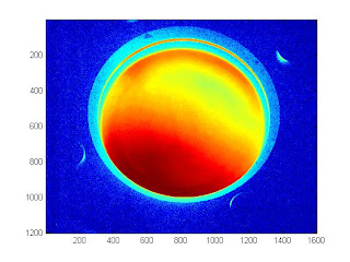
High dynamic range image using imagesc

Code Listing:

function hdr

% data

deltaT = 1./ [125 200 400 500 640 800 1000];

numpoints = 1000;

numrows = fix(rand(numpoints,1)*(1200-1))+1;

numcols = fix(rand(numpoints,1)*(1600-1))+1;

image_points = [numrows numcols];

% image_points = [510 875; %ok

% 606, 318;

% 540, 630;

% 942, 642;

% 790, 600; %ok

% 690 800]; %ok

% B(j) is the log delta t, or log shutter speed, for image j

Bj = log(deltaT);

% Z(i,j) is the pixel values of pixel location number i in image j

num_exposures = 7;

num_points = size(image_points, 1);

Zij = ones(num_points, num_exposures);

for i=1:1:num_exposures

filename = strcat(num2str(i), '.jpg');

current_image = rgb2gray(imread(filename));

for j=1:1:num_points

Zij(j,i) = current_image(image_points(j,1), image_points(j,2));

end

end

close all

for i=1:1:num_points

switch i

case 1

pattern = '+';

case 2

pattern = 'x';

case 3

pattern = 'o';

case 4

pattern = 's';

case 5

pattern = 'd';

case 6

pattern = '<';

case 7

pattern = '>';

end

plot(Zij(i,:)',Bj, pattern);

hold on

end

%

save data2.mat Zij Bj

load data2.mat

l = 10;

close all

[g,lE]=gsolve(Zij,Bj,l,@w);

image1 = rgb2gray(imread('1.jpg'));

new_hdr = uint8(zeros(size(image1)));

for i=1:1:7

current_file = rgb2gray(imread(strcat(num2str(i), '.jpg')));

new_hdr = new_hdr + current_file;

end

new_hdr = new_hdr ./ i;

% figure, imshow(new_hdr);

lnEi_temp = g(image1(:)+1) + Bj(1);

lnEi = reshape(lnEi_temp, size(image1,1), size(image1,2));

imwrite(uint8(lnEi), 'output.jpg');

figure,imshow(lnEi, []);

colormap(gray);

figure, imagesc(lnEi);

figure, plot(g);

end

% gsolve.m ? Solve for imaging system response function

%

% Given a set of pixel values observed for several pixels in several

% images with different exposure times, this function returns the

% imaging system’s response function g as well as the log film irradiance

% values for the observed pixels.

%

% Assumes:

%

% Zmin = 0

% Zmax = 255

%

% Arguments:

%

% Z(i,j) is the pixel values of pixel location number i in image j

% B(j) is the log delta t, or log shutter speed, for image j

% l is lamdba, the constant that determines the amount of smoothness

% w(z) is the weighting function value for pixel value z

%

% Returns:

%

% g(z) is the log exposure corresponding to pixel value z

% lE(i) is the log film irradiance at pixel location i

%

function [g,lE]=gsolve(Z,B,l,w)

n = 256;

A = zeros(size(Z,1)*size(Z,2)+n+1,n+size(Z,1));

b = zeros(size(A,1),1);

%% Include the data?fitting equations

k = 1;

for i=1:size(Z,1)

for j=1:size(Z,2)

wij = w(Z(i,j)+1);

A(k,Z(i,j)+1) = wij; A(k,n+i) = -wij; b(k,1) = wij * B(j);

k=k+1;

end

end

%% Fix the curve by setting its middle value to 0

A(k,129) = 1;

k=k+1;

%% Include the smoothness equations

for i=1:n-2

A(k,i)=l*w(i+1); A(k,i+1)=-2*l*w(i+1); A(k,i+2)=l*w(i+1);

k=k+1;

end

%% Solve the system using SVD

x = A\b;

g = x(1:n);

lE = x(n+1:size(x,1));

function d = w(Zint)

Zmin = 1;

Zmax = 255;

Zmid = (Zmin + Zmax)/2.0;

if Zint <= Zmid

d = (Zint - Zmin);

else

d = (Zmax - Zint);

end

return;

I give myself a grade of 10 for accomplishing the objectives and learning how to pass functions in Matlab. (yey! =)

References:

[1] "Recovering High Dynamic Range Radiance Maps from Photographs," P.E. Debevec, J. Malik, University of California, Berkeley

[2] High Dynamic Range Activity Sheet, Dr. Maricor Soriano